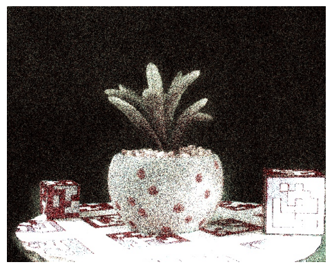
Pseudo-RGB Sensor Characterization
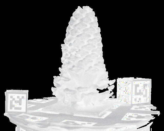
To characterize the pseudo-RGB image sensor, we first localized the camera pose of a query RGB photo of the scene using COLMAP.
To characterize the pseudo-RGB image sensor, we first localized the camera pose of a query RGB photo of the scene using COLMAP. Next, we use the closest corresponding ground truth hyperspectral image of the scene. We then used an RGB image of the scene (captured from a traditional camera) and identified K key points with varying color intensities. We used the corresponding hyperspectral intensities from the ground truth hyperspectral image for each keypoint to compute the per-keypoint pixel-level error. This error measures the difference between the RGB pixel values and the predicted pseudo-RGB intensities.
The error function is defined as follows:
\[ \mathcal{L} = \sum_{i,j} \lVert \mathbf{I}^{\mathrm{RGB}}_{i,j} - \mathbf{R} \, \mathbf{I}^{\mathrm{HS}}_{i,j} \rVert_2^2 \]
where \( \mathbf{R} \in \mathbb{R}^{3 \times N} \) represents the pseudo-RGB transformation matrix, \( \mathbf{I}^{\mathrm{RGB}}_{i,j} \in \mathbb{R}^3 \) is the \((i, j)\) pixel of the query image, and \( \mathbf{I}^{\mathrm{HS}}_{i,j} \in \mathbb{R}^{N} \) is the corresponding pixel in the ground truth hyperspectral image. The pseudo-RGB transformation matrix is split into three \(N \times 1\) vectors: \( \mathbf{r}(\lambda), \mathbf{g}(\lambda), \mathbf{b}(\lambda) \).
To simulate the behavior of an RGB sensor, we apply the pseudo-RGB transformation matrix as follows:
\[ \hat{\mathbf{I}}^{\mathrm{RGB}}_{i,j} = \begin{bmatrix} \mathbf{r}(\lambda) & \mathbf{g}(\lambda) & \mathbf{b}(\lambda) \end{bmatrix}^{\!T} \, \mathbf{I}^{\mathrm{HS}}_{i,j} \]
where \( \hat{\mathbf{I}}^{\mathrm{RGB}} \) denotes the simulated pseudo-RGB image.
Ablation Studies
We conduct comprehensive ablation studies to analyze the contribution of different components in our DD-HGS framework.
Positional Encoding
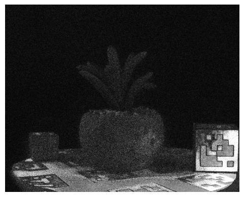
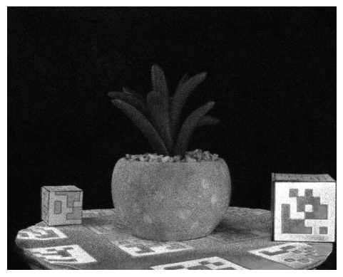
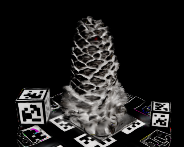
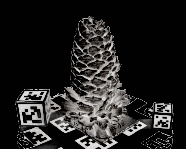
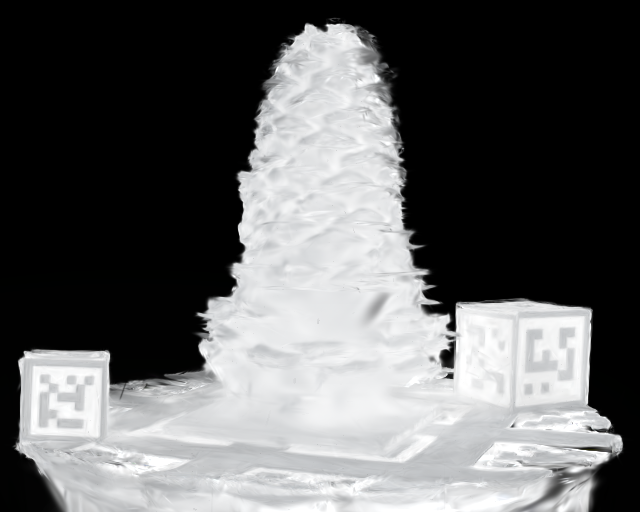
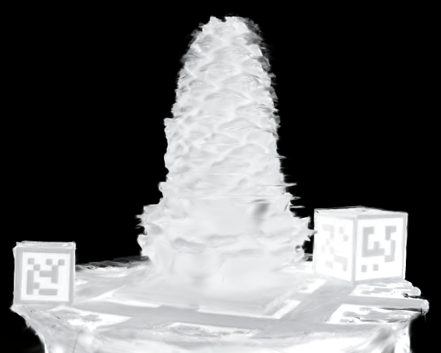
As shown in the table above and the figure below, the absence of positional embeddings (No Position) results in a significant loss of geometric structure and reflective details, particularly in the central regions and beyond-visual-range wavelengths of the Pinecone scene. The rendered details appear blurred and fail to represent fine textures accurately. To isolate the effect of positional encoding, all experiments in this study were conducted without the diffusion module.
Introducing positional embeddings (L = 5) significantly improves the rendering of finer reflective details and geometric accuracy, as evident in the sharper edges and clearer representation of reflective regions in the scene. However, further increasing the number of positional embeddings from L = 5 to L = 10 provides only marginal improvements, with relatively small enhancements in continuity and fidelity. This highlights that while positional embeddings are critical for wavelength encoding, increasing them beyond a certain threshold yields diminishing returns in terms of rendering quality.
| Method | Pinecone | Anacampserous | Caladium | Average | ||||
|---|---|---|---|---|---|---|---|---|
| PSNR ↑ | SSIM ↑ | PSNR ↑ | SSIM ↑ | PSNR ↑ | SSIM ↑ | PSNR ↑ | SSIM ↑ | |
| No PE | 18.31 | 0.8424 | 22.84 | 0.7681 | 20.18 | 0.8691 | 20.44 | 0.8265 |
| L = 5 | 22.13 | 0.8496 | 23.04 | 0.7716 | 20.54 | 0.8732 | 21.90 | 0.8315 |
| L = 10 (Ours) | 22.18 | 0.8497 | 23.05 | 0.7703 | 20.66 | 0.8738 | 21.96 | 0.8313 |

Spectral Loss
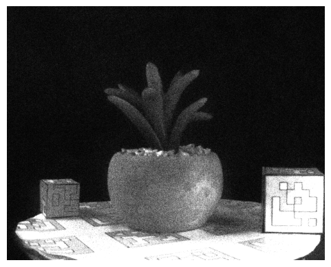
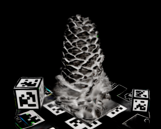
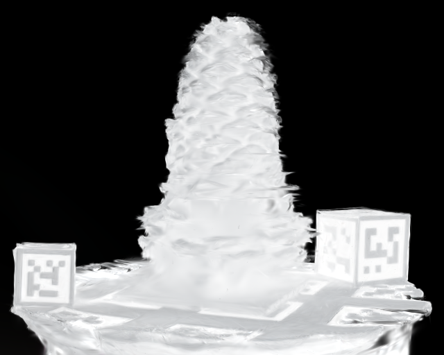
As shown in the table and figure below, the choice of Spectral Loss (SL) weight has a significant impact on rendering quality. To isolate the effect of spectral loss, all experiments in this section are conducted without the diffusion model. When the SL weight is set to 0.1, the rendered details in the central portion of the Pinecone plant are visible but lack refinement, and the reflective properties are not accurately captured.
Increasing the SL weight to 0.2 leads to a noticeable improvement in rendering accuracy. The finer details, particularly in the central portion, are better defined, and the reflective regions exhibit improved fidelity. However, further increasing the SL weight to 0.3 yields diminishing returns and degrades rendering quality, over-darkening the central region and obscuring fine details.
| \(w_3\) | Pinecone | Anacampserous | Caladium | Average | ||||
|---|---|---|---|---|---|---|---|---|
| PSNR ↑ | SSIM ↑ | PSNR ↑ | SSIM ↑ | PSNR ↑ | SSIM ↑ | PSNR ↑ | SSIM ↑ | |
| 0.1 | 22.06 | 0.8493 | 22.99 | 0.7692 | 20.56 | 0.8731 | 21.87 | 0.8305 |
| 0.3 | 22.05 | 0.8497 | 22.81 | 0.7673 | 20.56 | 0.8744 | 21.81 | 0.8305 |
| 0.2 (Ours) | 22.18 | 0.8497 | 23.05 | 0.7703 | 20.66 | 0.8738 | 21.96 | 0.8312 |
Diffusion Steps
We examine the effect of varying the number of diffusion steps on the final performance. Compared to vanilla 3DGS, the application of our hyperspectral diffusion module significantly improves both spectral accuracy (lower SAM) and visual sharpness (higher PSNR and SSIM). By varying the number of diffusion steps, we observe that the model with 1000 steps consistently yields the best results across all the hyperspectral scenes.
| Steps | Pinecone | Anacampserous | Caladium | |||
|---|---|---|---|---|---|---|
| PSNR ↑ / SSIM ↑ | SAM ↓ / RMSE ↓ | PSNR ↑ / SSIM ↑ | SAM ↓ / RMSE ↓ | PSNR ↑ / SSIM ↑ | SAM ↓ / RMSE ↓ | |
| 10 | 24.91 / 0.9305 | 0.0624 / 0.0272 | 27.63 / 0.9418 | 0.0263 / 0.0435 | 27.42 / 0.9321 | 0.0271 / 0.0450 |
| 500 | 25.03 / 0.9332 | 0.0593 / 0.0251 | 28.02 / 0.9450 | 0.0250 / 0.0416 | 27.61 / 0.9349 | 0.0255 / 0.0420 |
| 1000 | 25.11 / 0.9347 | 0.0572 / 0.0244 | 28.57 / 0.9490 | 0.0247 / 0.0381 | 27.86 / 0.9362 | 0.0248 / 0.0312 |
Implementation Details
We implement our framework based on the 3D Gaussian Splatting implementation from Nerfstudio, and train our model for 60,000 steps. The wavelength encoder is trained jointly with 3D Gaussians using an Adam optimizer with \(\epsilon = 10^{-15}\). For 3D Gaussian parameters, we set the learning rate as \(1.6 \times 10^{-4}\), while for the wavelength encoder, we set the learning rate as \(1.6 \times 10^{-5}\).
For the diffusion model, we leverage a timestep conditioned U-Net which is a hierarchical encoder-decoder structure with residual connections and time-step embeddings. The hyperspectral input is progressively downsampled through convolution blocks with increasing channel dimensions, and subsequently upsampled to reconstruct the output. We empirically set the weights \(w_1\), \(w_2\), \(w_3\), and \(w_4\) as 0.4, 0.2, 0.1 and 0.3 respectively to balance different loss terms. For spectral loss, we set \(\alpha = 0.5\) and \(\beta = 0.5\). All experiments are conducted on one NVIDIA A40 GPU.
Runtime and Memory Benchmarks
We provide a detailed evaluation and comparison of the runtime and memory consumption of DD-HGS and other methods.
We provide a detailed evaluation and comparison of the runtime and memory consumption of DD-HGS and other methods. The table below reports training time per iteration, peak GPU memory, number of Gaussians and inference speed in frames per second (FPS).
We observed that the vanilla 3DGS model is the most efficient, achieving inference speeds above 75 FPS. The inclusion of the diffusion module increases memory usage and reduces inference speed to around 2.4 FPS. Despite this, DD-HGS still performs much faster than NeRF-based methods in both training and rendering speed. In sum, DD-HGS achieves a good balance between reconstruction performance and computational efficiency.
| Method | Train. Time (s) | GPU Mem (GB) | Gaussians | FPS ↑ |
|---|---|---|---|---|
| NeRF | 821 | 10.9 | - | 0.13 |
| Hyper-NeRF | 261 | 10.6 | - | 0.5 |
| 3DGS | 0.48 | 7.6 | 112,350 | 75.2 |
| 3DGS + Diffusion | 1.23 | 19.1 | 134,024 | 2.4 |
| 3DGS + Spectral Loss | 0.85 | 11.8 | 128,910 | 54.3 |
| 3DGS + Wavelength Encoder | 0.87 | 12.2 | 129,704 | 52.7 |
| DD-HGS (Ours) | 1.25 | 19.4 | 134,472 | 2.2 |
Evaluation Metrics
For comparison, we utilize the following metrics to quantitatively evaluate the model performance. Peak Signal-to-Noise Ratio (PSNR) measures pixel-level reconstruction quality. Structural Similarity Index Measure (SSIM) evaluates perceived structural similarity. Spectral Angle Mapper (SAM) quantifies spectral distortion in radians. Root Mean Squared Error (RMSE) captures absolute error between predicted and ground truth. Finally, Frames Per Second (FPS) denotes the number of rendered frames per second by the method.
Autoencoder Baselines on BaySpec Dataset
To evaluate the performance of traditional low-dimensional latent reconstruction models on hyperspectral data, we train an autoencoder and a variational autoencoder on three representative plant scenes (Pinecone, Anacampserous, Caladium) from the BaySpec dataset.
Autoencoder: We firstly train an autoencoder baseline using a U-Net-style encoder-decoder architecture. The autoencoder baseline consistently underperforms in both spatial and spectral metrics (PSNR, SSIM, SAM), demonstrating its inferior performance on preserving fine-grained spectral features across view-dependent geometry and material variations. Notably, SAM scores are significantly worse than those of 3DGS or our proposed DD-HGS method, validating that simple bottleneck-based reconstructions are inadequate for hyperspectral consistency.
Variational Autoencoder: Due to the high channel dimensionality of hyperspectral inputs (up to 141 bands), the VAE's latent sampling and reconstruction pipeline ran out of memory in our experiment. This further reinforces the need for spatially conditioned and spectrally aware architectures, such as DD-HGS, that can scale to such domains.
| Method | Pinecone | Anacampserous | Caladium | |||||||||
|---|---|---|---|---|---|---|---|---|---|---|---|---|
| PSNR ↑ | SSIM ↑ | RMSE ↓ | SAM ↓ | PSNR ↑ | SSIM ↑ | RMSE ↓ | SAM ↓ | PSNR ↑ | SSIM ↑ | RMSE ↓ | SAM ↓ | |
| Autoencoder | 10.45 | 0.2841 | 0.2763 | 0.1984 | 9.90 | 0.2291 | 0.3068 | 0.2145 | 11.02 | 0.3187 | 0.2634 | 0.1862 |
| 3DGS | 21.40 | 0.8487 | 0.0640 | 0.0912 | 22.61 | 0.7622 | 0.0682 | 0.0451 | 20.40 | 0.8729 | 0.0615 | 0.0583 |
| 3DGS + Diffusion | 24.50 | 0.9285 | 0.0292 | 0.0621 | 27.10 | 0.9401 | 0.0417 | 0.0264 | 26.92 | 0.9263 | 0.0439 | 0.0249 |
| DD-HGS (Ours) | 25.11 | 0.9347 | 0.0244 | 0.0572 | 28.57 | 0.9490 | 0.0381 | 0.0247 | 27.86 | 0.9362 | 0.0417 | 0.0224 |